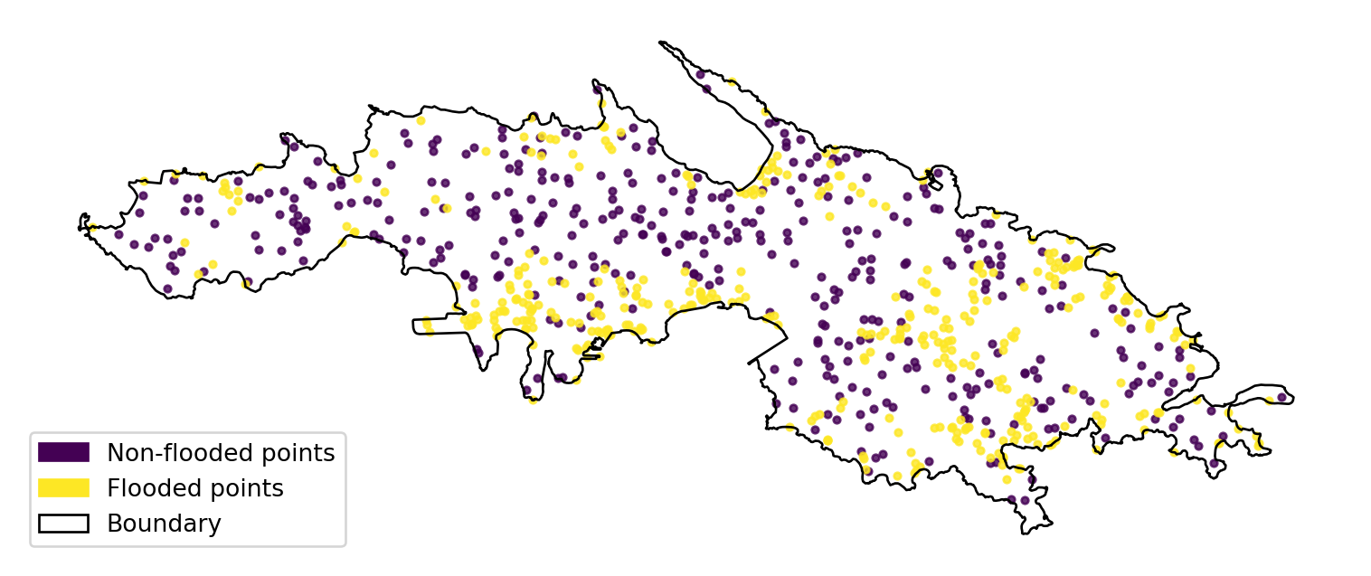
Flood Inventory and Feature Selection

Flood Inventory Construction

A synthetic flood inventory is built by sampling flooded points inside FEMA/USVI high-risk zones (FLD_ZONE in {VE, AE, AO, A}) and non-flooded points from the residual safe area, further constrained to elevations greater than 5 m according to the DEM. After removing overlaps, 400 flooded and 400 non-flooded points were retained. Each point carries a binary label (1 = flooded, 0 = non-flooded). The resulting map shows flooded and non-flooded points across the island of St. Thomas. This balanced inventory is then split 70/30 for training and testing the machine-learning flood susceptibility model. For detailed code on how the flood inventory was processed, please refer to this repository.

Code

import matplotlib.pyplot as plt
import matplotlib.patches as mpatches
import numpy as np
from pathlib import Path
import geopandas as gpd

images_dir = Path("images")
images_dir.mkdir(exist_ok=True)

# reuse existing boundary/inventory; load boundary if missing
try:
    boundary  # noqa: F821
except NameError:
    boundary = gpd.read_file("data/processed/st_thomas_boundary.geojson")

# inventory must already exist in memory (with 'label' column)
# if not, rerun the sampling step that builds pos_pts/neg_pts and concatenates them
if "inventory" not in globals():
    raise RuntimeError("inventory not found; run the sampling step first")

cmap = plt.cm.viridis
colors = cmap(np.linspace(0, 1, 3))
neg_color, pos_color = colors[0], colors[2]

pos_gdf = inventory[inventory["label"] == 1]
neg_gdf = inventory[inventory["label"] == 0]

fig, ax = plt.subplots(figsize=(8, 10))
fig.patch.set_alpha(0.0)
ax.set_facecolor("none")

boundary.boundary.plot(ax=ax, color="black", linewidth=1, label="Boundary")
neg_gdf.plot(ax=ax, color=neg_color, markersize=8, alpha=0.8, label="Non-flooded points")
pos_gdf.plot(ax=ax, color=pos_color, markersize=8, alpha=0.8, label="Flooded points")

ax.set_axis_off()
legend_patches = [
    mpatches.Patch(color=neg_color, label="Non-flooded points"),
    mpatches.Patch(color=pos_color, label="Flooded points"),
    mpatches.Patch(facecolor="none", edgecolor="black", label="Boundary"),
]
ax.legend(handles=legend_patches, loc="lower left")
plt.tight_layout()

Figure 1: Flood inventory map of St Thomas

Feature Selection

To capture the environmental, hydrologic, and anthropogenic conditions shaping flood susceptibility on St. Thomas, the feature selection process incorporates 14 predictors derived from elevation, terrain, land cover, hazard zones, and proximity indicators. Land cover plays a particularly important role. This land cover dataset includes 13 distinct land cover classes, spanning developed areas (low-, medium-, and high-intensity; and open space), which represent gradations of built environments and impervious surfaces. Natural land cover classes are also well represented, including Forest, Shrubland, and Rangeland, which capture vegetation structure and ecological variation across the island, and additional categories such as water, wetland, cultivated land, barren surfaces, seaside areas, and airport land. Land cover classes were spatially joined to each inventory point using geopandas.sjoin, and one-hot encoded using pandas.get_dummies, allowing categorical surface types to be incorporated into the Random Forest model. These steps ensure that each observation contains a consistent set of hydrologic and land-based predictors representing both natural and built environmental processes. In addition, raster-based variables—such as elevation, slope, and distance to ghuts, were extracted at each sample location using a coordinate, based sampling function (rasterio.sample). The tsunami exposure variable was encoded as a binary indicator by testing whether each point fell within the designated tsunami zone polygon.

Collectively, these features capture the core mechanisms shaping flood behavior on small tropical islands. Areas closer to ghuts are more vulnerable to channel overflow; lower elevations and flatter terrain accumulate surface water; steeper slopes enhance runoff and reduce ponding; and developed land, with extensive impervious surfaces, tends to exhibit higher flood sensitivity compared to vegetated or permeable surfaces. By encoding these relationships numerically, the resulting predictor matrix provides a comprehensive representation of the physical and anthropogenic drivers of flood susceptibility across St. Thomas.

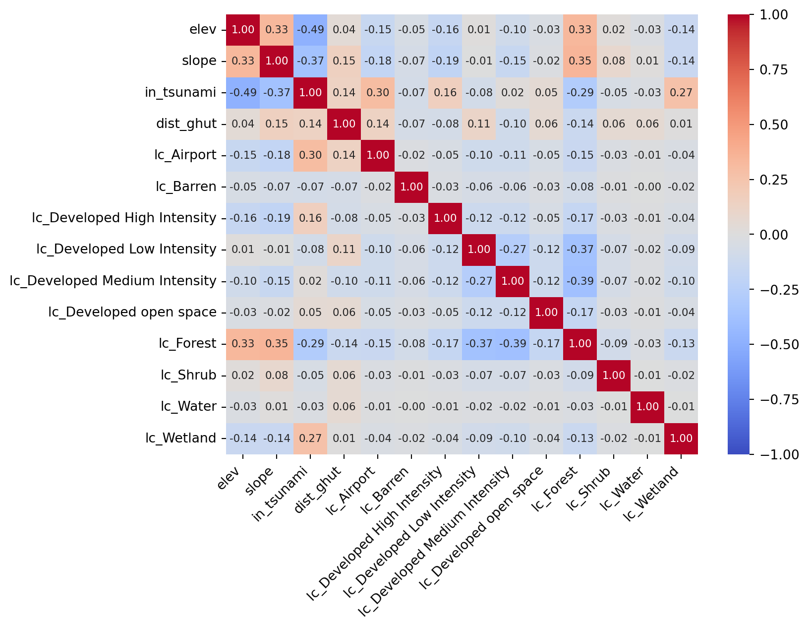
To minimize multicollinearity, Pearson correlation coefficients were computed among all selected predictors. The absolute values of all coefficients remained below 0.8, consistent with prior literature noting that |PCC| > 0.8 may introduce problematic collinearity.

Code

import os
from pathlib import Path

images_dir = Path("images")
images_dir.mkdir(exist_ok=True)

# ML: Random Forest
feature_cols = [c for c in inventory.columns 
                if c not in ["geometry", "label", "index_right",
                             "rain_annual_mean", "rain_max_month","lc_Rangeland"]]
X = inventory[feature_cols].values
y = inventory["label"].values

# Train-test split
X_train, X_test, y_train, y_test = train_test_split(
    X, y, test_size=0.3, random_state=42, stratify=y
)

# Convert training set to DataFrame for correlation analysis
train_df = pd.DataFrame(X_train, columns=feature_cols)

# Plot correlation heatmap WITH numeric values
plt.figure(figsize=(8, 6))
sns.heatmap(
    train_df.corr(),
    cmap="coolwarm",
    vmin=-1,
    vmax=1,
    annot=True,
    fmt=".2f",
    annot_kws={"size": 8}
)
plt.xticks(rotation=45, ha="right")
plt.yticks(rotation=0)
plt.show()